


Choosing lamination thickness: 0.23, 0.27 or 0.30 mm is about more than 0.07 mm
Thinner electrical steel cuts eddy-current loss, but it also adds layers, stamping strokes, die wear and stacking-factor loss. How thickness affects core loss, how frequency sets the lower limit, and how to choose between 0.23, 0.27 and 0.30 mm.
“Can we switch from 0.27 to 0.23 mm?” is one of the questions we hear most at the quotation stage. The reasoning is usually sound: thinner steel, lower loss, more efficiency margin. But it covers only half of the decision.
In our Hunan plant, a 0.27 mm grain-oriented coil is being cut to length while inspection measures thickness variation across the sheet, not the nominal thickness printed on the mill certificate. At the stacking table next to it, a 0.23 mm core needs about 435 layers for 100 mm of stack height; the same height in 0.35 mm takes about 286. The two cores look the same, but core loss, labour hours and material price are all different.
Thickness is the specification field most often filled in “by default”: the grade is chosen and the thickness follows, or the drawing is copied from the last revision. Yet it decides three things at once — core loss, processing and cost. This article answers the questions we are asked most.
The short answer
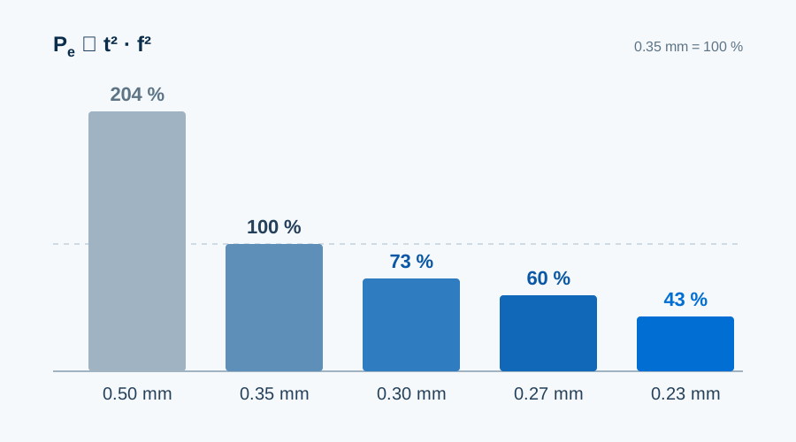
- Thickness mainly changes eddy-current loss, and it does so with the square: going from 0.35 to 0.27 mm takes the eddy-current part to about 60%; to 0.23 mm, about 43%.
- Total core loss improves less than that, because hysteresis loss does not fall with thickness.
- The higher the frequency, the more a thin gauge is worth. 50/60 Hz transformers do not need to chase thinness; motors running at 400 Hz and above cannot do without it.
- Thin gauges have a price: more layers, more stamping strokes, faster die wear and a lower stacking factor.
- A grade name is only a maximum. Measured loss can differ by a class between batches of the same grade, so compare measured values, not grade names.
Thicknesses in this article are nominal values. For a specific coil, the measured thickness and thickness variation on the mill certificate apply.
Thickness, mil and gauge
Electrical steel thickness means the thickness of a single lamination — not the coil, and not the core stack height. Two units are common: millimetres and mils (1 mil = 0.001 inch = 0.0254 mm). Trade documents round mil values, so “9 mil” is an approximation of 0.2286 mm, not an exact 0.23 mm.
| Metric | Exact mil | Common label (mil) | Typical use |
|---|---|---|---|
| 0.18 mm | 7.1 | 7 | Large power transformers, GO |
| 0.20 mm | 7.9 | 8 | High-frequency thin NGO |
| 0.23 mm | 9.1 | 9 | Low-loss transformers, GO |
| 0.27 mm | 10.6 | 11 | Mainstream power transformers, GO |
| 0.30 mm | 11.8 | 12 | Distribution transformers, GO |
| 0.35 mm | 13.8 | 14 | High-efficiency motors (NGO), transformers (GO) |
| 0.50 mm | 19.7 | 20 | General industrial motors, NGO |
| 0.65 mm | 25.6 | 26 | Generators, low-cost motors, NGO |
Gauge numbers were never defined consistently across standards and materials, and in older mill catalogues a gauge could even be an order code rather than a physical thickness. Write the value instead: “0.27 mm, tolerance to standard X” is clearer than “27 gauge”. If a contract still uses gauge, add the millimetre value next to it.
GO and NGO use different thickness ranges
Grain-oriented steel (GO) is used in transformers, where the magnetic path is fixed and the loss budget is tight, so it is made thin: 0.18, 0.23, 0.27, 0.30 and 0.35 mm are the common commercial sizes, with 0.23–0.30 mm the main range for distribution and power transformers. Non-oriented steel (NGO) is used in rotating machines with very different frequencies and cost structures, so its range is wider: 0.35, 0.50 and 0.65 mm are common, and thin grades of 0.20 mm and below serve high-speed and EV traction motors.
The grade name usually encodes loss class and thickness. M235-35A means non-oriented steel with a maximum loss of 2.35 W/kg (1.5 T, 50 Hz) at 0.35 mm. Grain-oriented names follow another pattern: Baosteel B30P105 is 0.30 mm, high-permeability, with a guaranteed loss of 1.05 W/kg at 1.7 T, 50 Hz.
The most common misreading: GO is rated at P17/50 and NGO at P15/50. The flux densities differ, so the two numbers cannot be ranked against each other. Putting a 0.90 W/kg grain-oriented grade and a 3.0 W/kg non-oriented grade in one league table means nothing — they do different jobs.
Why thickness works on the square
Core loss has three parts. Hysteresis loss rises in proportion to frequency and depends on purity, grain size and internal stress; annealing improves it and cutting stress worsens it. Eddy-current loss rises with the square of frequency and the square of thickness and falls with resistivity — this is the part thickness controls. Excess (anomalous) loss comes from domain-wall motion; it is smaller but not negligible.
At 50 Hz and around 0.30 mm, the split is roughly 60% hysteresis, 30% eddy current and 10% excess. That decides the remedy: when eddy current dominates, go thinner; when hysteresis dominates, change the grade or anneal. Getting this the wrong way round wastes money.
By the square rule, 0.35 → 0.27 mm takes the eddy-current part to (0.27/0.35)² ≈ 60%, 0.35 → 0.23 mm to about 43%, and 0.50 → 0.35 mm to about 49%. Total loss always improves by less, because hysteresis does not follow. That is why one project measures 8% lower loss after moving from 0.35 to 0.27 mm and another only 4%: grade, flux density, frequency and processing state make the difference.
Frequency magnifies all of this. Eddy-current loss grows with the square of frequency, hysteresis only linearly, so at 400 Hz or 1 kHz eddy current is often the largest part. Skin depth is another measure: for silicon steel with a resistivity of about 0.5 μΩ·m it is roughly 0.3–0.4 mm near 1 kHz — already the size of a lamination — and about 0.1 mm at 10 kHz. These are order-of-magnitude estimates, not design inputs.
A worked example: what is 0.15 W/kg worth?
Take a distribution transformer core with 1.5 tonnes of grain-oriented steel and two materials whose measured losses differ by 0.15 W/kg. The difference is 225 W per transformer, about 1,970 kWh per year over 8,760 hours, and about 39,000 kWh over 20 years. Multiply by your electricity tariff to set it against the price difference of the thinner material.
The calculation has limits: 0.15 W/kg is an assumption and varies widely between grades; real flux density and frequency differ from test conditions, so the difference cannot be scaled linearly; and the lower stacking factor, extra stamping strokes and shorter die life of thin material are not included. Use it to compare options and judge orders of magnitude, not as an energy-saving promise.
Frequency sets the lower limit
| Application | Typical frequency | Common thickness | Why |
|---|---|---|---|
| Large power transformers | 50 / 60 Hz | 0.23–0.30 mm | Lifetime efficiency first; thin GO cuts no-load loss directly |
| Standard industrial motors | 50 / 60 Hz | 0.35–0.50 mm | Balance of cost and performance; material and processing cost weigh heavily |
| High-efficiency / inverter-fed motors | 50–400 Hz | 0.20–0.35 mm | Inverter harmonics add high-frequency loss that standard gauges cannot cover |
| EV traction motors, aerospace | 400–1000+ Hz | 0.10–0.27 mm | Eddy current becomes the main loss; it drives range, power density and cooling |
This table is a starting point, not an answer. A 50/60 Hz transformer can be built with 0.35 mm, but no-load loss and the efficiency class must be checked again; an EV motor will run on 0.35 mm, but efficiency and temperature rise at high speed will suffer.
Our own range: HXES processes material from 0.18 to 0.50 mm. Gauges of 0.10–0.15 mm come from specific mills, have narrower processing windows and are not stock items; for these we confirm the material source first and then discuss processing.
0.23, 0.27 or 0.30 mm?
| Thickness | Typical choice | Main trade-off |
|---|---|---|
| 0.23 mm | Loss-sensitive transformer cores, some high-efficiency designs | Low eddy-current loss, but higher price, more layers and a narrow stamping window |
| 0.27 mm | Balanced low-loss and manufacturable designs | Compromise between performance and processing; common in mainstream power transformers |
| 0.30 mm | General transformers, reactors and some industrial uses | Easy to process and lower cost; higher eddy-current share than thinner gauges |
We suggest deciding in this order rather than picking a thickness first:
- Set the loss budget. Work back from the efficiency target to the allowed no-load loss and then to W/kg. Choosing the thickness first and checking afterwards usually means rework.
- Compare measured values. Use the mill certificate values of the two materials, not the grade names. A low-loss 0.23 mm grade and a high-permeability 0.27 mm grade can each win.
- Ask the production line. Press tonnage, die clearance, feed accuracy and stacking method must handle the gauge reliably; otherwise laboratory values stay on paper.
- Add up the total. Material price, stamping strokes, die cost, stacking hours and 20 years of loss energy belong in one comparison.
In short, 0.23 mm is not automatically better than 0.27 mm, nor 0.27 mm better than 0.30 mm. Thickness is only part of a grade; talking about thickness without the loss class reads only half the specification.
The hidden costs of thin gauges
Stamping: clearance and strokes
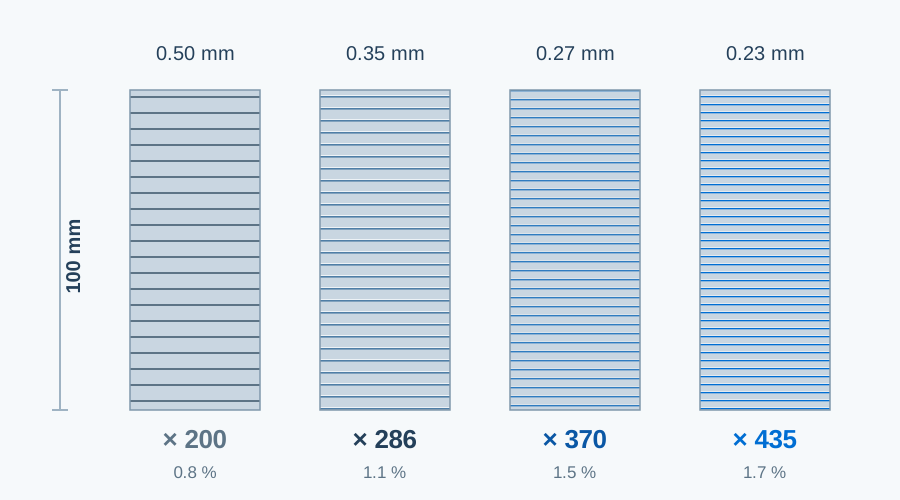
Thin material needs smaller absolute die clearance, with tighter demands on clearance uniformity, edge condition and feed accuracy, so dies need regrinding more often — a structural effect, not a question of operator skill. Strokes rise too: 100 mm of stack takes about 286 layers at 0.35 mm and about 435 at 0.23 mm, roughly half as many strokes again.
Burr: 0.02 mm is a hard limit
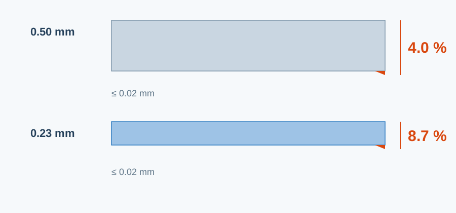
Burrs bridge adjacent sheets, short-circuit the eddy-current paths, heat locally and damage the coating, which ends as abnormal temperature rise. Our slitting and cutting limit is 0.02 mm. On 0.50 mm material that leaves margin; on 0.23 mm it is close to the edge — the burr grows from 4% to 8.7% of the thickness. Judge burr relative to thickness, not only as an absolute value.
Cutting: the damaged zone scales up
Laser and water-jet cutting suit samples and small batches, but the zone next to the cut loses magnetic quality. Its depth is roughly fixed, so halving the thickness doubles its share of the cross-section: an edge effect negligible at 0.50 mm can cost a few per cent of the magnetic path at 0.23 mm. Stamping remains the most stable route for series production; a laser-cut sample validates the design, not series performance, and the project plan should say so.
Stacking: layers, coating and stacking factor
Coatings are thin — usually 1–3 μm per side — but they add up. At 2 μm per side, coating takes about 1.7% of stack height at 0.23 mm, 1.1% at 0.35 mm and 0.8% at 0.50 mm, so a 100 mm stack of 0.23 mm holds almost 2 mm less steel, which the design must compensate. More layers also magnify alignment, staggering and clamping-force variation; holding a stacking factor of 0.95–0.97 with thin material needs better fixtures and procedures.
How thickness is held: at the mill, X-ray or laser gauges scan the strip and feed deviations back to the automatic gauge control of the rolling mill. At our end, incoming coils are re-measured, slit coils are sampled and the first stamped part is checked. Thin material is especially sensitive to thickness variation, which shows up directly in stack height.
Why the “same grade” can carry different prices
Material within one grade does not perform identically. Pricing by grade name — one price for M235-35A, another for M270-35A — assumes it does, and in transformers, where every 0.01 W/kg counts, that assumption fails. Thickness, measured loss and test conditions together form a comparable basis. When you compare offers:
- ask for the measured values of the batch (P17/50 or P15/50, B8, thickness, thickness variation, coating) with the quotation;
- state the guaranteed values and the acceptance method, including sampling position and pass criteria, in the contract;
- compare material cost per core plus 20 years of no-load loss energy, not only the price per tonne — the hidden part is often the larger one.
Frequently asked questions
Why not use the thinnest gauge everywhere?
Thin steel lowers eddy-current loss but raises stamping difficulty, die wear, layer count and labour. Gains and costs have to be weighed for each project; thin is not free.
Is thicker always cheaper at 50 Hz? What about 0.65 mm?
Where frequency and loss targets are not demanding, thicker steel is often more economical, but not automatically best. Many standard industrial motors use 0.50 or even 0.65 mm NGO because cost and processing advantages outweigh the extra loss.
How thick are motor laminations usually?
Standard industrial motors mostly use 0.35–0.50 mm NGO; high-speed, EV and high-frequency motors move to 0.20–0.27 mm to hold down eddy-current loss as frequency rises.
Is 0.23 mm always better than 0.27 mm?
No. Thickness only affects the eddy-current part; total loss depends on grade, measured value, flux density and frequency. A 0.27 mm grade measuring 0.90 W/kg can beat a 0.23 mm grade measuring 0.95 W/kg.
In closing
Choosing thickness means solving three constraints together: how low the loss must be, how thin the line can process reliably, and how high a price the budget can carry. In the projects we see, problems rarely come from choosing too thick or too thin; they come from not putting the three on one sheet.
Fix the loss budget, compare measured values, then have the production line confirm it can make it. If you are deciding between 0.23, 0.27 and 0.30 mm, send us the drawing or grade and we will lay out the measured values, processing window and total cost of both options side by side.
Data ranges are taken from public standards and common grade information for orientation and selection; actual grade performance follows the mill certificate and the technical agreement. The worked example is an order-of-magnitude estimate, not an energy-saving promise.

